How to use MIRR Function in Excel

MIRR in excel is an in-build financial function used to calculate the modified internal rate of return for the cash flows supplied with a period. This function takes the set of initial investment or loan values and a set of net income values with the interest rate paid on initial amount including the interest earned from reinvestment of earned amount and returns the MIRR (modified internal rate of return) as output

Syntax:= MIRR (values, finance_rate, reinvest_rate)

The MIRR function syntax has the following arguments:

• Values    Required. An array or a reference to cells that contain numbers. These numbers represent a series of payments (negative values) and income (positive values) occurring at regular periods.
  • Values must contain at least one positive value and one negative value to calculate the modified internal rate of return. Otherwise, MIRR returns the #DIV/0! error value.
  • If an array or reference argument contains text, logical values, or empty cells, those values are ignored; however, cells with the value zero are included.
• Finance_rate    Required. The interest rate you pay on the money used in the cash flows.

• Reinvest_rate    Required. The interest rate you receive on the cash flows as you reinvest them.

Example: Let’s look at some Excel MIRR function examples and explore how to use the MIRR function as a worksheet function in Microsoft Excel:

Consider an initial loan amount of 10,000,000 as initial investment amount (loan amount) with an interest rate of 10% yearly and you have earned an interest rate of 12% from the reinvested income. In MIRR the loan amount or initial investment amount is always considered as (-ve) value.

Syntax:  =MIRR($B$1:B3,$B$8,$B$9)

Result:

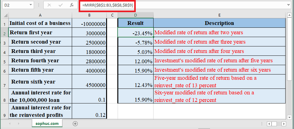
Based on the Excel spreadsheet above, the following MIRR examples would return:

Note:

• Values must contain at least one negative value & one positive value to calculate the modified internal rate of return. Otherwise, MIRR returns the #DIV/0! error
• If an array or reference argument contains empty cells, text or logical values, those values are ignored
• #VALUE! error occurs if any of the supplied arguments is not a numeric value or non-numeric
• Initial investment needs to be in negative value, otherwise, the MIRR Function will return an error value (#DIV/0! Error)
• MIRR Function takes into consideration both the cost of the investment (finance_rate) and the interest rate received on cash reinvestment (reinvest_rate).
• Main Difference between MIRR & IRR is MIRR considers the interest received on the reinvestment of cash, whereas the IRR does not consider it.
• If n is the number of cash flows in values, frate is the finance_rate, and rrate is the reinvest_rate, then the formula for MIRR is: